This simulation studies boron diffusion and clustering. Comparison with experiments (Pelaz et al., 1997) is also carried out. Silicon is self-implanted in a Silicon sample with a narrow boron spike (4.5 x 1019 cm-3) grown by Molecular Beam Epitaxy (MBE) near the top surface. Si self implant is performed at 40 keV with a dose of 9 x 1013 cm-2 and a dose rate of 1 x 10¹² ions cm-2 s-1. After implantation, the sample is annealed. An analysis of the defect evolution is carried out, taking into account the boron profiles, boron clusters, etc. As epitaxial growth is not included as a command in UVAS, Boron spike is simulated by reading a narrow Boron profile into the silicon sample.
A name must be assigned to Object Name and Client Data.
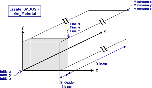
Maximum x: 350 nm
Maximum y: 100 nm
The values of the parameters Minimum x, Minimum y and Minimum z must be zero.
Material: SiOxide
Initial x: 0
Initial y: 0
Initial z: 0
Final x: 1.5 nm
Final y: 10000 nm
It is important to point out that the values of Final y and Final z are greater than the values of Maximum y and Maximum z in Create_DADOS command. In this way, the new material layer fits the previously defined simulation box. In this case, a thin layer of Silicon Oxide with a thickness of 1.5 nm on top of the Si is included.
After these two commands, the following simulation box has been created:
This comand is used for visualization purposes. UVAS introduces experimental data (Pelaz et al., 1997) from several DA2IN files in order to compare them with the simulation results. In this particular simulation, there are used five different files: one for the evolution of boron concentration, and the rest for comparing boron profile in different moments.
Input data series 1: ...\B9e13_5s.da2in
Input data series 2: ...\B9e13_50s.da2in
Input data series 3: ...\B9e13_500s.da2in
Input data series 4: ...\B9e13_2100s.da2in
A B spike profile file is read. The B spike has a width of 20 nm (from 107 to 127 nm) and a concentration of 4.5 x 1019 cm-3.
Time: 0 s
Start Output Time (s): 0.1 s
Snapshots per Decade: 10
UVAS starts the graph structure defined in the GPH file. As the simulation proceeds, UVAS takes different snapshots and the results are plotted on the screen.
Implant species: Silicon
Energy (keV): 40 keV
Tilt: 7°
Rotation: 45°
Dose: 9 x 1013 cm-2
Dose rate: 1 x 10¹² ions cm-2 s-1
Target Structure: Crystal
Initial Temperature: 26.85 °C
Final Temperature: 800 °C
The annealing process is divided in four parts in order to take a snapshot after each of them. This facilitates the comparison between simulation results and the experimental data previously introduced by Input_Data_Series command.
Initial Temperature: 800 °C
Final Temperature: 800 °C
Every annealing process has the same initial and final temperature but they have different times.
Time 1: 5 s
Time 2: 45 s
Time 3: 450 s
This simulation studies the behaviour of a 4.5 x 1019 cm-3 B spike after a 40 keV 9 x 1013 cm-2 Si implant and a 2100 s anneal at 800 °C.
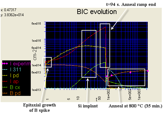
At the beginning, a B spike is grown by Molecular Beam Epitaxy (MBE). This spike consists of only substitutional B (Bs), since there are no defects, because it has been grown by MBE in the experiment. Then, Si is implanted at 40 keV with a dose of 9 x 1013 cm-2. The interstitial concentration increases and there occur many interactions between B and defects. This causes the formation of immobile B clusters. When the annealing process begins, point defects are recombined and some amorphous pockets are dissolved very soon, while others evolve to become {311} defects. During annealing, B TED (Transient Enhanced Diffusion) starts and the immobile B fraction do not increase. Finally, B has spread throughout the simulation box and the clusterized B spike remains immobile. Simulation evolution is shown in the following graph.
Next graph shows B evolution vs time.
The simulation can be divided in the following moments:
First of all, a B spike profile file is read. This B spike of 20 nm width and a concentration of 4.5 x 1019 cm-3 is implanted around a depth of 100 nm, simulating the experimental epitaxial growth. In this moment, this spike is only composed of substitutional B atoms, since there is no defect generation and Si has not yet been ion-implanted.

![]()
Once the B spike is in the silicon, 40 keV Si is implanted and the Si interstitials concentration increases. These point defects form amorphous pockets and their population becomes increasingly important. The implantation causes a very high supersaturation of Si interstitials and there are also many interactions between B atoms and defects, since free interstitials and vacancies are mobile during implantation at room temperature.
Next graph shows Si interstitial profile at the end of Si implantation, which is at 90 s.
Mobile B-I pair (Bi) are formed. Then, Bi may become substitutional B (Bs) if it interacts with a vacancy (Frank-Turnbull mechanism). On the other hand, Bi may form an immobile complex (BI2) through the interaction with an additional free interstitial.
During implantation, immobile B clusters are formed. Boron-interstitial clustering is observed only in the regions with a very high supersaturation of Si interstitials. The B cluster precursors consist of a B atom and several Si interstitials, such as BI2, and they are formed during Si implantation or in the early stages of the post-implant annealing. This species is immobile and helps the B clusters to grow, since it acts as a nucleation center. Then, BI2 capture additional Bi and, as a result, other B clusters are formed.
The following histogram shows the compositions of B clusters when Si implant have been finished. BI2 is predominant, though there are other configurations of B clusters (BnIm), such as B2I2 and B2I3.
There are different paths of formation of B clusters and all of them have different energies. The formation happens by the capture of additional Bi or by releasing a Si interstitial. These paths of formation and their energies are shown in the following figure (Pelaz et al., 1999).
Next graph shows B profile at the end of Si implantation. Most of the boron atoms are in boron-interstitial clusters (BIC), and a small fraction remains as point defect. Clusterized B atoms in the spike are immobile, while substitutional boron (point defect) can move by interaction with interstitials.
![]()
Once anneal begins, point defects are recombined, so the concentration of free interstitials drops very soon. Next graph shows the boron profile at 94 s, once the initial annealing ramp is finished. Boron in binary complex experiences a slight reduction. On the other hand, only non-clusterized B (PD) is able to diffuse, as can be seen in the graph. The formation of a mobile B-I pair due to the excess population of Si interstitials is the main reason of B TED.
![]()
During annealing at 800°C, there are three important topics to study: the broadening of B-interstitial cluster (BIC) profile, the B TED and the spreading and evolution of the compositions of B clusters.
First, the following graphs show the evolution of B profile during the annealing process. After a 2100 s anneal at 800 °C, BIC remains immobile and substitutional B diffuses throughout the simulation box. Moreover, the concentration of B in complex configuration decreases slowly along the simulation, because B clusters dissolve by releasing free interstitials.
These simulation results are in very good agreement with the experiments (red line in the graphs). At 5 s about 50% of B atoms are in clusters, while after 2100 s annealing, only 30% of B atoms remain in them. There is a slight reduction and some substitutional B atoms are released by B clusters. In addition, these Bs atoms experience TED.
B atoms in BICs are immobilized before any diffusion occurs, so there is no broadening of B cluster profile. On the other hand, there is an important B diffusion. Isolated B atoms bind to free interstitials and reach a high mobility state.
Regarding to interstitial profile, amorphous pockets start to dissolve and evolve into {311} defects. The interstitials emitted by amorphous pockets dissolution are the main cause of B diffusion. Interstitial B (Bi), which has a high mobility, is formed as a result of this interaction. Then, when amorphous pockets are dissolved, {311} defects also start to dissolve by releasing free interstitials which help B diffusion.
Next graph shows interstitials profile at 160 s. Almost all amorphous pockets are dissolved and most of interstitials are in {311} defects. On the other hand, BICs remain immobile and the concentration of interstitials in them has hardly decreased.
Next snapshot, taken at 500s, shows that {311} defects have disappeared, and only boron-interstitial clusters remain in the simulation box.
Referring to the evolution of the B clusters composition, all of them evolve into B3I when anneal begins. It is supposed that this configuration is the most stable because it does not evolve into other configuration and dissolves slowly. Next, the binary complex map at 100 s is detailed.
In very long anneals, BICs dissolve completely. All interstitials are emitted first, resulting in B-rich clusters. In this simulation, at the end of 35 min. anneal there are some B2 clusters.
![]()
![]() Pelaz, L., Jaraiz, M., Gilmer, G.
H., Gossman, H. J., Rafferty, C. S., Eaglesham, D. J. and Poate, J. M. "B
diffusion and clustering in ion implanted Si: The role of B cluster precursors".
Applied Physics Letters
70, 2285 (1997)
Pelaz, L., Jaraiz, M., Gilmer, G.
H., Gossman, H. J., Rafferty, C. S., Eaglesham, D. J. and Poate, J. M. "B
diffusion and clustering in ion implanted Si: The role of B cluster precursors".
Applied Physics Letters
70, 2285 (1997)
![]() Pelaz, L., Gilmer, G. H.,
Gossman, H. J., Rafferty, C. S., Jaraiz, M. and Barbolla, J. "B cluster
formation and dissolution in Si: A scenario based on atomistic modeling".
Applied Physics Letters
74, 2017 (1999)
Pelaz, L., Gilmer, G. H.,
Gossman, H. J., Rafferty, C. S., Jaraiz, M. and Barbolla, J. "B cluster
formation and dissolution in Si: A scenario based on atomistic modeling".
Applied Physics Letters
74, 2017 (1999)