The filters used in the RTTY program are of the IIR type. IIR means Infinite Impulse Response, which in turn, means that the filter is implemented using some kind of feedback. The general IIR filter algorithm is:
Where ![]() is the current input sample and
is the current input sample and ![]() is the current
output sample. As it can be seen, the current output sample depends on the previous
output samples, so here is the feedback.
is the current
output sample. As it can be seen, the current output sample depends on the previous
output samples, so here is the feedback.
The IIR filters are computer efficient, but they are very sensitive to coefficient accuracy and can become unstable. To avoid instability, the order of the filter must be low. Higher order filters are implemented by cascading lower order sections. In this program the filter section is order 2 and it is commonly called ``biquad''. The filter behavior is dictated by its own coefficients, and the calculation of these coefficients are the purpose of the digital filter design.
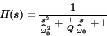
The filter design starts with a continuous-time version of the biquad filter
section, the resonant frequency, ![]() , is ``prewharped'' to
account for the further frequency response distortion. Then the Bilinear transform
is used to translate the continuous-time filter to a discrete-time version of
the filter, where its transfer function is written in terms of the Z transform.
Finally the filter coefficients are derived from the discrete-time transfer
function.
, is ``prewharped'' to
account for the further frequency response distortion. Then the Bilinear transform
is used to translate the continuous-time filter to a discrete-time version of
the filter, where its transfer function is written in terms of the Z transform.
Finally the filter coefficients are derived from the discrete-time transfer
function.
In the following example a bandpass resonator is designed. The filter parameters
are its resonant frequency ![]() , and its quality factor
, and its quality factor ![]() .
In order to account for the error introduced by the Bilinear transform, the
resonant frequency is prewharped, so the used resonant frequency is:
.
In order to account for the error introduced by the Bilinear transform, the
resonant frequency is prewharped, so the used resonant frequency is:
![]() ,
where
,
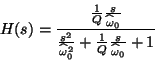
where ![]() is the sampling frequency. The continuous-time transfer function,
written in the Laplace transform terms, is:
is the sampling frequency. The continuous-time transfer function,
written in the Laplace transform terms, is:
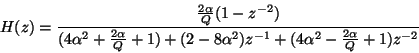
Then, we use the Bilinear transformation to obtain an approximate discrete-time
equivalent transfer function. The Bilinear transform is merely the replacement
of ``![]() '' by ``
'' by ``
![]() '' in equation
1.2. The new transfer function is then:
'' in equation
1.2. The new transfer function is then:
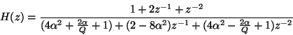
where
![]()
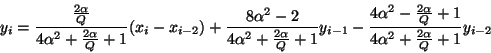
Then, the recurrence algorithm is derived taking into account that
![]() ,
and that
,
and that ![]() is represented in the time domain by an
is represented in the time domain by an ![]() clock
cycle delay. From equation 1.3 we obtain:
clock
cycle delay. From equation 1.3 we obtain:
And finally, by matching equation 1.4 with equation 1.1, the filter coefficients are easily obtained.
These bandpass resonators are used to split the signal into a mark & space bands in the very front-end of the demodulator, but the demodulator also includes a low-pass filter, which is divided into two biquad sections giving a total stopband attenuation of 80 dB/dec. Each section has the following transfer functions:
And the recurrence algorithm is: